

Rob Smedley has explained the Massey’s method used to find out the Top 50 fastest F1 drivers from 1983 until 2019 season.
F1 together with Amazon Web Services released an initial list of the Top 10 Fastest Drivers’ from 1983 until 2019 season, where Ayrton Senna beat Michael Schumacher and Lewis Hamilton. Later on, a list of Top 20 drivers was released with 10 more names.
Looking at the backlash, Smedley has explained the method used to devise the list, wherein they have now released further names from P21 until P50. The Brit revealed of Amazon SageMaker app where they used Massey’s method to prepare the whole list.
In a write-up, Smedley detailed on how they found out the F1 Fastest Driver:
Quantifying driver pace using qualifying data –
We define pace as a driver’s lap time during qualifying sessions. Driver race performance depends on a large number of factors, such as weather conditions, car setup (such as tires), and race track. F1 qualifying sessions are split into three sessions: the first session eliminates cars that set a lap time in 16th position or lower, the second eliminates positions 11–15, and the final part determines the grid position of 1st (pole position) to 10th. We use all qualification data from the driver qualifying sessions to construct Fastest Driver.
Lap times from qualifying sessions are normalized to adjust for differences in race tracks, which enables us to pool lap times across different tracks. This normalization process equalizes driver lap time differences, helping us compare drivers across race tracks and eliminating the need to construct track-specific models to account for track alterations over time.
Another important technique is that we compare qualifying data for drivers on the same race team (such as Aston Martin Red Bull Racing), where teammates have competed against each other in a minimum of five qualifying sessions. By holding the team constant, we get a direct performance comparison under the same race conditions while controlling for car effects.
Differences in race conditions (such as wet weather) and rule changes (such as rule impacts) leads to significant variations in driver performances. We identify and remove anomalous lap time outliers by using deviations from median lap times between teammates with a 2-second threshold. For example, let’s compare Daniel Ricciardo with Sebastian Vettel when they raced together for Red Bull in 2014.
During that season, Ricciardo was, on average, 0.2 seconds faster than Vettel. However, the average lap time difference between Ricciardo and VetteI falls to 0.1 seconds if we exclude the 2014 US Grand Prix (GP), where Ricciardo was more than 2 seconds faster than Vettel on account of Vettel being penalized to comply with the 107% rule (which forced him to start from the pit lane).
Constructing Fastest Driver –
Building a performant ML model starts with good data. Following the driver qualification data aggregation process, we construct a network of teammate comparisons over the years, with the goal of comparing drivers across all teams, seasons, and circuits. For example, Sebastian Vettel and Max Verstappen have never been on the same team, so we compare them through their respective connections with Daniel Ricciardo at Red Bull.
Ricciardo was, on average, 0.18 seconds slower than Verstappen during the 2016–2018 seasons while they were at Red Bull. We remove outlier sessions, such as the 2018 GPs in Bahrain, where Ricciardo was quicker than Verstappen by large margins because Verstappen didn’t get past Q1 due to a crash. If each qualifying session is assumed to be equally important, a subset of our driver network including only Ricciardo, Vettel, and Verstappen yields Verstappen as the fastest driver: Verstappen was 0.18 seconds faster than Ricciardo, and Ricciardo 0.1 seconds faster than Vettel.
Using the full driver network, we can compare all driver pairings to determine the faster racers. Going back to Heikki Kovalainen, let’s look at his years in the McLaren team against Lewis Hamilton. The qualifying speaks volumes with the median difference of just 0.1 seconds per lap. Kovalainen doesn’t have the same number of World Championships as Hamilton, but his qualifying statistics speak for themselves—the model has ranked him high because of his consistent qualifying performance throughout his career.
An algorithm called the Massey’s method (a form of linear regression) is one of the core models behind the Insight. Fastest Driver uses Massey’s method to rank drivers by solving for a set of linear equations, where each driver’s rating is calculated as their average lap time difference against teammates. Additionally, when comparing ratings of teammates, the model uses features like driver strength of schedule normalized by the number of interactions with the driver. Overall, the model places high rankings to drivers who perform extraordinarily well against their teammates or perform well against strong opponents.
Our goal is to assign each driver a numeric rating to infer that a driver’s competitive advantage relative to other drivers assuming the expected margin of lap time difference in any race is proportional to the difference in a driver’s true intrinsic rating. For the more mathematically inclined reader: let xj represent each of all drivers and rj represent the true intrinsic driver ratings. For every race, we can predict the margin of the lap time advantage or disadvantage (yi) between any pair of two drivers as:
![]()
In this equation, xj is +1 for the winner and -1 for the loser, and ei is the error term due to unexplained variations. For a given set of m game observations and n drivers, we can formulate an (m * n) system of linear equations:
![]()
Driver ratings (r) is a solution to the normal equation via linear regression:
![]()
Lightweight and flexible deployment with Amazon SageMaker –
To deliver the insights from Fastest Driver, we implemented Massey’s method on a Python web server. One complication was that the qualifying data consumed by the model is updated with fresh lap times after every race weekend. To handle this, in addition to the standard request to the web server for the rankings, we implemented a refresh request that instructs the server to download new qualifying data from Amazon Simple Storage Service (Amazon S3).
We deployed our model web server to an Amazon SageMaker model endpoint. This makes sure that our endpoint is highly available, because multi-instance Amazon SageMaker model endpoints are distributed across multiple Availability Zones by default, and have automatic scaling capabilities built in. As an additional benefit, the endpoints integrate with other Amazon SageMaker features, such as Amazon SageMaker Model Monitor, which automatically monitors model drift in an endpoint. Using a fully-managed service like Amazon SageMaker means our final architecture is very lightweight. To complete the deployment, we added an API layer around our endpoint using Amazon API Gateway and AWS Lambda.
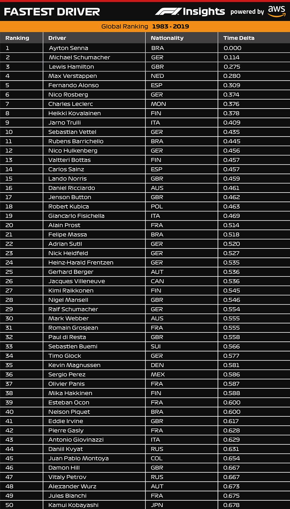
Here’s the full Top 50 list of F1 drivers:
Here’s the defence on Heikki Kovalainen and Jarno Trulli
Here’s the Top 20 list of F1 Fastest Driver